Data processing is an essential step in data science and machine learning, and one of the most common techniques used to prepare data is transformation. Transformation allows us to modify the distribution of a variable, making it more amenable to statistical analysis or machine learning algorithms. One commonly used transformation is the Box-Cox transformation, which is particularly useful when dealing with non-normal data. In this blog post, we will focus on the Box-Cox transformation of 1 + x, provide examples, and discuss exemplary use cases with synthetic, generated datasets. We will also provide Python code snippets to illustrate the process.
The Box-Cox Transformation
The Box-Cox transformation is a technique used to transform non-normal data into normal data. It was developed by statisticians George Box and David Cox in 1964. The transformation involves applying a power function to the data, which can be expressed as:
where y is the transformed variable, x is the original variable, and lambda is the transformation parameter. When lambda is equal to zero, the transformation reduces to the logarithmic transformation. In general, the optimal value of lambda is estimated from the data.
The Box-Cox transformation of 1 + x is a specific form of the Box-Cox transformation that is used when the data contains negative values. The transformation can be expressed as:
The Box-Cox transformation of 1 + x is particularly useful when dealing with count data, as it helps to normalize the data and reduce the impact of outliers.
Note: the Box-Cox transformation requires that the data are positive. If your arbitrary distribution produces negative values, you may need to add a constant to shift the data to be positive.
Example 1: Synthetic Data
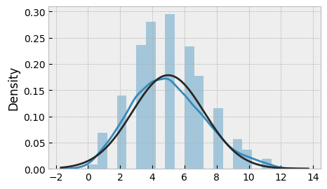
To illustrate the Box-Cox transformation of 1 + x, we will generate a synthetic dataset using NumPy. Let's generate 1000 data points from a Poisson distribution with a mean of 5:
import numpy as np

np.random.seed(42)
x = np.random.poisson(5, 1000)
If we plot the histogram of x, we can see that the data is right-skewed:
import matplotlib.pyplot as plt
from scipy.stats import norm
import seaborn as sns

plt.style.use("bmh")
_ = plt.subplots(figsize=(5, 3))
sns.distplot(x, fit=norm);
plt.show()

We can apply the Box-Cox transformation of 1 + x to the data using the boxcox1p function from SciPy:
from scipy.stats import boxcox1p

xt = boxcox1p(1 + x, 0)
The boxcox1p function returns two values: the transformed data xt, and the optimal value of lambda lmbda. In this case, we set lambda to zero, which corresponds to the logarithmic transformation.
If we plot the histogram of the transformed data, we can see that it is closer to a normal distribution:
plt.hist(xt, bins=20)
plt.show()
Example 2: Generated Data
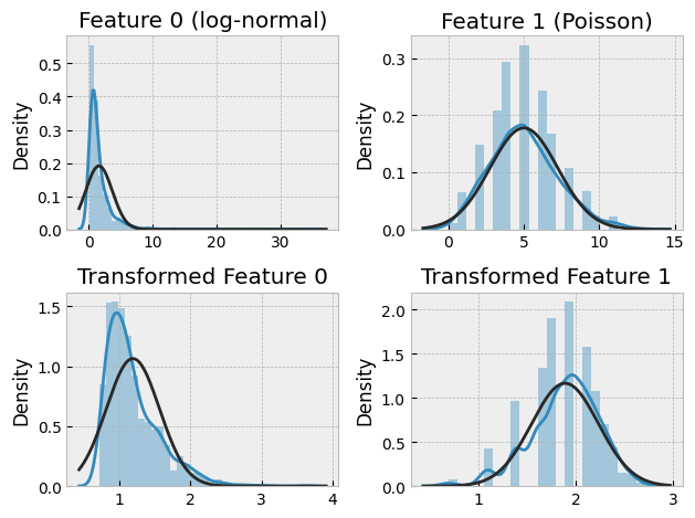
In this example, we will generate a dataset with two features, one of which is generated from a log-normal distribution, and the other from a Poisson distribution. We will then apply the Box-Cox transformation of 1 + x to both features and compare the results.
[from sklearn.datasets import make_regression

np.random.seed(42)
X, y = make_regression(n_samples=1000, n_features=2, noise=10)

X[:, 0] = np.exp(X[:, 0])
X[:, 1] = np.random.poisson(X[:, 1])](<import numpy as np

# Set seed for reproducibility
np.random.seed(123)

# Generate 1000 data points for each feature
lognormal_data = np.random.lognormal(mean=0, sigma=1, size=1000)
poisson_data = np.random.poisson(lam=5, size=1000)
# Combine the two features into a single dataset
X = np.column_stack((lognormal_data, poisson_data))
We can apply the Box-Cox transformation of 1 + x to the first and second feature using the boxcox1p function:
# Apply the Box-Cox transformation of 1 + x to both features
lognormal_transformed = boxcox1p(1 + lognormal_data, 0)
poisson_transformed = boxcox1p(1 + poisson_data, 0)

# Combine the two features into a single dataset
Xt = np.column_stack((lognormal_transformed, poisson_transformed))
If we plot the histograms of the original and transformed features, we can see that the transformed features are closer to a normal distribution:
plt.subplot(2, 2, 1)
sns.distplot(X[:, 0], fit=norm)
plt.title("Feature 0 (log-normal)")

plt.subplot(2, 2, 2)
sns.distplot(X[:, 1], fit=norm)
plt.title("Feature 1 (Poisson)")

plt.subplot(2, 2, 3)
# plt.hist(Xt[:,0], bins=20)
sns.distplot(Xt[:, 0], fit=norm)
plt.title("Transformed Feature 0")

plt.subplot(2, 2, 4)
sns.distplot(Xt[:, 1], fit=norm)
plt.title("Transformed Feature 1")

plt.tight_layout()
plt.show()
Use Cases
The Box-Cox transformation of 1 + x is particularly useful when dealing with count data or data with a large number of zeros, as it helps to normalize the data and reduce the impact of outliers. Here are some exemplary use cases:
Customer behavior analysis
If you are analyzing customer behavior, you may be interested in counting the number of times customers visit your website or interact with your products. Count data is typically right-skewed and can benefit from the Box-Cox transformation of 1 + x to normalize the data.
Financial data analysis
Financial data often exhibits high levels of volatility and may contain outliers. The Box-Cox transformation of 1 + x can help to reduce the impact of outliers and make the data more amenable to statistical analysis or machine learning algorithms.
Medical data analysis
Medical data often contains a large number of zeros, which can make it difficult to analyze. The Box-Cox transformation of 1 + x can help to normalize the data and make it more suitable for statistical analysis or machine learning algorithms.
Conclusion
The Box-Cox transformation of 1 + x is a useful technique for normalizing non-normal data, particularly count data or data with a large number of zeros. In this blog post, I provided examples of the Box-Cox transformation of 1 + x using synthetic and generated datasets, and discussed exemplary use cases. I also provided Python code snippets to illustrate the process.