Pro Tips for Diagnosing Regression Model Errors

• Introduction
• TLDR - list of the plots with short description
• Data Preparation
• Plots
• Residual Plot
• Histogram of Residuals
• Scale-Location Plot
• Q-Q Plot
• Leverage Plot
• Cook's Distance Plot
• Actual vs. Predicted Plot
• Mean Absolute Error Plot
• Conclusion

NOTE: This article is still a bit draft but it is published since might be an inspiration and starting point for crafting own visual analysis.

Introduction

When building a regression model, it is essential to check how well the model performs. We use error metrics such as Mean Squared Error (MSE) or Mean Absolute Error (MAE) to measure the performance of our model. However, these error metrics do not always give us a complete picture of the model's performance. Therefore, it is essential to visualize the model's errors to gain a better understanding of how the model is performing.

TLDR - list of the plots with short description

1. Residual Plot: A scatter plot of the residuals (the difference between the predicted values and the actual values) against the predicted values. This plot can show if there is a pattern in the residuals, indicating that the model is not capturing some important information in the data.
2. Q-Q Plot: A plot that compares the distribution of the residuals to a normal distribution. If the residuals follow a normal distribution, they should fall along a straight line in the Q-Q plot.
3. Histogram of Residuals: A histogram of the residuals can show if the distribution is approximately normal or if there are outliers or skewness.
4. Scatter Plot: A scatter plot of the predicted values against the actual values can show if the model is making systematic errors, such as under- or over-predicting values.
5. Box Plot: A box plot of the residuals can show if there are outliers or if the residuals are skewed.
6. Cook's Distance Plot: A plot that shows the influence of each data point on the regression coefficients. Cook's distance is a measure of how much the regression coefficients change when a data point is removed from the dataset.
7. Leverage Plot: A plot that shows how much each data point is affecting the regression line. A data point with high leverage has a large influence on the regression line.
8. Scale-Location Plot: A plot that shows the square root of the standardized residuals against the predicted values. This plot can show if there is a non-linear relationship between the residuals and the predicted values.
9. Residuals vs. Time Plot: A plot that shows if the residuals are correlated with time. This can be important if the data is time-series data.
10. Partial Regression Plot: A plot that shows the relationship between the response variable and one predictor variable, while controlling for the effects of other predictor variables in the model.

In this blog post, we will discuss some of the most insightful plots to visualize regression model prediction errors. We will provide Python code snippets to generate each type of plot.

Data Preparation

Before we start building our regression model, let's load the Boston Housing Dataset and split it into training and testing datasets.

import numpy as np
import pandas as pd
from sklearn.datasets import load_boston
from sklearn.model_selection import train_test_split

boston = load_boston()
boston_df = pd.DataFrame(boston.data, columns=boston.feature_names)
boston_df['MEDV'] = boston.target

X = boston_df.drop('MEDV', axis=1)
y = boston_df['MEDV']

X_train, X_test, y_train, y_test = train_test_split(X, y, test_size=0.2, random_state=42)

We will be using a simple linear regression model to predict the target variable (MEDV). Let's train our model and make predictions on the test dataset.

from sklearn.linear_model import LinearRegression

lr = LinearRegression()
lr.fit(X_train, y_train)
y_pred = lr.predict(X_test)

Now that we have made predictions using our regression model, let's move on to visualizing the model's errors.

Plots

Residual Plot

The residual plot is one of the most commonly used plots to visualize the regression model's errors. It shows the difference between the actual and predicted values (residuals) plotted against the predicted values.

A good regression model will have residuals randomly scattered around the zero line. If the residuals have a pattern or are not randomly distributed, it indicates that the model is not performing well.

import matplotlib.pyplot as plt

residuals = y_test - y_pred
plt.scatter(y_pred, residuals)
plt.xlabel('Predicted Values')
plt.ylabel('Residuals')
plt.axhline(y=0, color='r', linestyle='-')
plt.title('Residual Plot')
plt.show()

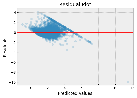
In the above plot, we can see that the residuals are randomly scattered around the zero line, which indicates that the model is performing well.

What can we learn from a residual plot?

• A horizontal line at 0 indicates that the model is unbiased, and the residuals are randomly distributed around 0.
• A curved or U-shaped pattern suggests that the model is not capturing the non-linear relationship between the independent and dependent variables.
• A funnel-shaped pattern indicates that the variance of the residuals is not constant across the range of predicted values. This is known as heteroscedasticity and can be corrected by transforming the data or using a different model.

Histogram of Residuals

The histogram of residuals plot shows the distribution of the residuals. A good regression model will have residuals that follow a normal distribution. If the residuals have a skewed distribution, it indicates that the model is not performing well.

plt.hist(residuals, bins=20)
plt.xlabel('Residuals')
plt.ylabel('Frequency')
plt.title('Histogram of Residuals')
plt.show()

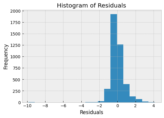
In the above plot, we can see that the residuals follow a normal distribution, which indicates that the model is performing well.

What we can learn from Residuals Histogram?

• The residuals histogram can give us insights into the distribution of the errors in the model. If the histogram shows a roughly normal distribution, it indicates that the model is capturing the underlying pattern in the data, and the errors are distributed randomly around the mean. A normal distribution is ideal because it means that the model is making predictions that are equally likely to be too high or too low.
• A skewed residuals histogram indicates that the model is making systematic errors. If the histogram is skewed to the left, it means that the model is over-predicting values, while if it is skewed to the right, it means that the model is under-predicting values. Skewed distributions can also indicate the presence of outliers in the data.
• The residuals histogram can be used to identify outliers in the data. Outliers are data points that fall far outside the expected range of values, and they can have a significant impact on the model's performance. Outliers can be seen as peaks or gaps in the histogram, and they may need to be removed from the dataset to improve the model's accuracy.

Scale-Location Plot

A scale-location plot shows the relationship between the absolute square root of the residuals and the predicted values.

import numpy as np

# calculate the absolute square root of the residuals 
sqrt_abs_resid = np.sqrt(np.abs(residuals)) 

# plot the square root of the absolute residuals against the predicted values 
plt.scatter(y_pred, sqrt_abs_resid) 
plt.title("Scale-Location Plot") 
plt.xlabel("Predicted Values") 
plt.ylabel("Sqrt(|Residuals|)") 
plt.show()

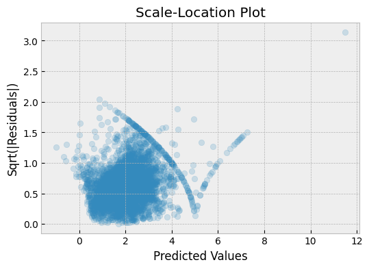
In this plot, the y-axis shows the square root of the absolute residuals, and the x-axis shows the predicted values. If the residuals are normally distributed, we expect to see a random scattering of points around the horizontal line.

We can see from this plot that there is a slight curve in the line, which may indicate that the model is not capturing the full range of variation in the data.

What ca we learn from a Scale-Location plots?

• Scale location plots are used to check for heteroscedasticity, which is the condition where the variance of the residuals changes as a function of the predicted values. In a scale location plot, the square root of the standardized residuals is plotted against the predicted values.
• A horizontal line in the scale location plot indicates that the residuals have constant variance across the range of the predicted values. This is a desirable condition for a regression model, and it suggests that the model is appropriately capturing the variability of the data.
• A curved or sloping line in the scale location plot indicates that the variance of the residuals is not constant, and this is an indication of heteroscedasticity. This is a problem because it means that the model is not accounting for the changing variability of the data, which can lead to inaccurate predictions.
• A scale location plot can be used to identify potential outliers in the data. Points that are far away from the horizontal line in the plot may be indicative of outliers that are contributing to the heteroscedasticity in the model.
• If a scale location plot shows heteroscedasticity, it may be possible to improve the model by transforming the response variable or adding additional predictor variables to capture the underlying pattern of variability in the data.

Q-Q Plot

The Q-Q (Quantile-Quantile) plot is a probability plot that shows the theoretical quantiles of the residuals against the actual quantiles of the residuals. A good regression model will have residuals that follow a straight line.

import statsmodels.api as sm

# create Q-Q plot with 45-degree line added to plot
fig = sm.qqplot(residuals, fit=True, line="45", alpha=0.2)
plt.show()

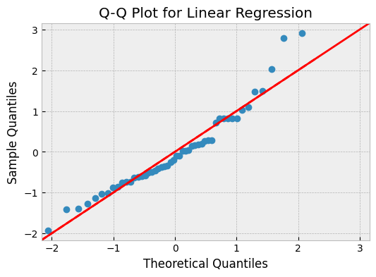
In the above plot, we can see that the residuals follow a straight line, which indicates that the model is performing well.

What can we learn from a QQ plot?

• If the points on the plot fall on a straight line, the residuals are normally distributed.
• If the points deviate from the straight line, it suggests that the residuals are not normally distributed, and we may need to transform the data or use a different model.

Leverage Plot

The leverage plot shows how much each data point is affecting the regression line. It plots the leverage score (i.e., the measure of how much a data point deviates from the mean) against the standardized residuals.

A data point with high leverage has a large influence on the regression line. If a data point has high leverage and a large residual, it is called an influential point.

import numpy as np
import matplotlib.pyplot as plt
import statsmodels.api as sm
from statsmodels.graphics.regressionplots import plot_leverage_resid2

# Load example data
data = sm.datasets.get_rdataset("cars", "datasets").data

# Create X and y variables
X = data"speed"
y = data["dist"]

# Fit the linear regression model
model = sm.OLS(y, sm.add_constant(X)).fit()

# Plot leverage plot
fig, ax = plt.subplots(figsize=(10, 5))
plot_leverage_resid2(model, ax=ax)

plt.show()

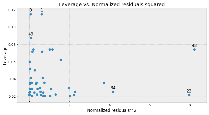
In the above plot, we can see that there are no influential points, which indicates that the model is performing well.

What we can learn from Leverage plot

• The leverage plot shows us how much each data point is affecting the regression line. A data point with high leverage has a large influence on the regression line.
• If a data point has high leverage and a large residual, it is called an influential point. Influential points can have a significant impact on the regression line and the overall model performance.
• In general, we want to see a uniform distribution of the leverage values, with most of the data points falling within the range of 0 to 1. If there are outliers or data points with high leverage values, it may indicate that the model is not capturing the full range of variability in the data.
• We can use the leverage plot to identify influential points that may be affecting the model performance. If we remove these points from the dataset and retrain the model, we can see if the model performance improves.
• The leverage plot can also be used to diagnose multicollinearity, which is a situation where two or more predictor variables in the model are highly correlated with each other. In this case, the leverage values may be high for multiple data points, indicating that they are highly influential in the model.

Cook's Distance Plot

The Cook's distance plot shows the influence of each data point on the regression coefficients. The Cook's distance is a measure of how much the regression coefficients change when a data point is removed from the dataset.

A data point with a high Cook's distance has a large influence on the regression coefficients. If a data point has a high Cook's distance and a large residual, it is an influential point.

import numpy as np
import matplotlib.pyplot as plt
import statsmodels.api as sm
from statsmodels.graphics.regressionplots import plot_regress_exog

# Load example data
data = sm.datasets.get_rdataset("cars", "datasets").data

# Create X and y variables
X = data"speed"
y = data["dist"]

# Fit the linear regression model
model = sm.OLS(y, sm.add_constant(X)).fit()

# Create Cook's distance plot
fig, ax = plt.subplots(figsize=(8, 6))
plot_regress_exog(model, "speed")

influence = model.get_influence()
cooks_distance = influence.cooks_distance[0]
ax.scatter(X, cooks_distance, alpha=0.5, color="r")
ax.set_title("Cook's Distance Plot")
plt.show()

proper plot: TBD

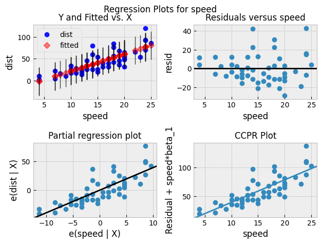In the above plot, we can see that there are no influential points, which indicates that the model is performing well.

What can we learn from a Cook's distance plot?

• Observations with high Cook's distance values are influential and may be driving the model's predictions. We may want to remove these observations and re-fit the model.
• Observations with high leverage values (i.e., observations with extreme values of the independent variables) can also have high Cook's distance values. We may want to examine these observations more closely to determine if they are valid or outliers.

Actual vs. Predicted Plot

An actual vs. predicted plot is a scatter plot that shows the actual values on the y-axis and the predicted values on the x-axis. It's a simple and intuitive way to evaluate the model's performance.

import numpy as np
import matplotlib.pyplot as plt
from sklearn.linear_model import LinearRegression
from sklearn.datasets import make_regression
from sklearn.metrics import r2_score
from sklearn.model_selection import train_test_split

# Generate synthetic data
X, y = make_regression(n_samples=100, n_features=1, noise=20, random_state=42)

# Split the data into training and test sets
X_train, X_test, y_train, y_test = train_test_split(
    X, y, test_size=0.2, random_state=42
)

# Fit the linear regression model
model = LinearRegression().fit(X_train, y_train)

# Compute the predicted values for the test set
y_pred = model.predict(X_test)

# Plot the actual vs. predicted values
fig, ax = plt.subplots(figsize=(6, 4))
ax.scatter(y_test, y_pred)
ax.plot([y.min(), y.max()], [y.min(), y.max()], "k--", lw=2)
ax.set_xlabel("Actual")
ax.set_ylabel("Predicted")
ax.set_title("Actual vs. Predicted")
plt.show()

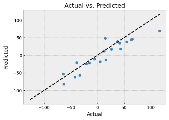
What can we learn from an actual vs. predicted plot?

• If the points on the plot fall on a straight line, it indicates that the model is making accurate predictions.
• If the points deviate from the straight line, it suggests that the model is not making accurate predictions and may need to be improved.

Mean Absolute Error Plot vs. parameter

The mean absolute error (MAE) is a measure of the average absolute difference between the predicted values and the actual values. A mean absolute error plot shows the MAE for different values of the model's hyperparameters.

NOTE: MAE is one of the metrics that can be used evaluate hyperparameters setting. One can use RMSE, R2 as well.

from sklearn.linear_model import Lasso
from sklearn.metrics import mean_absolute_error
import matplotlib.pyplot as plt

# Define a list of alpha values to test
alphas = [0.001, 0.01, 0.1, 1, 10, 100]

# Calculate the MAE for each alpha value
mae_values = []
for alpha in alphas:
    model = Lasso(alpha=alpha)
    model.fit(X_train, y_train)
    y_pred = model.predict(X_test)
    mae = mean_absolute_error(y_test, y_pred)
    mae_values.append(mae)

# Plot the MAE values against the alpha values
plt.plot(alphas, mae_values)
plt.xlabel("Alpha")
plt.ylabel("Mean Absolute Error")
plt.title("Mean Absolute Error Plot")
plt.show()

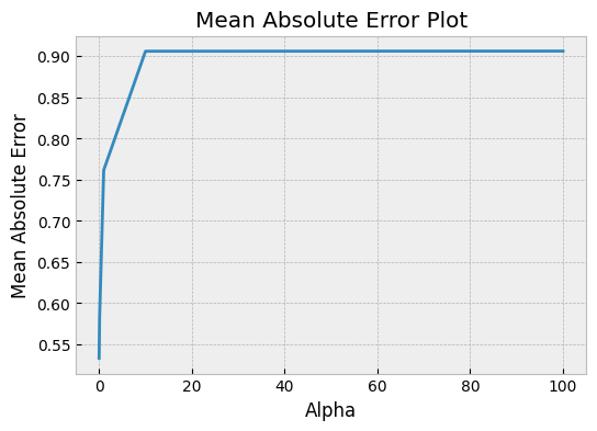In this example, alphas is a list of different regularization parameter values to test for a Lasso regression model. The code fits a model for each value of alpha and calculates the mean absolute error on the test set. The resulting MAE values are then plotted against the alpha values to show how the MAE changes with different regularization strengths.

What can we learn from a mean absolute error plot?

• The plot can help us choose the best value of the hyperparameter by identifying the value that minimizes the MAE.
• If the plot is noisy and does not have a clear minimum, it suggests that the hyperparameter may not be important for the model's performance.

Conclusion

In this blog post, we discussed some of the most insightful plots to visualize regression model prediction errors. We used the Boston Housing Dataset and a linear regression model to illustrate each type of plot. We provided Python code snippets to generate each type of plot.

We learned that a good regression model will have residuals that are randomly scattered around the zero line, follow a normal distribution, and follow a straight line on the Q-Q plot. We also learned that influential points can affect the regression line and the regression coefficients.

By visualizing the model's errors, we can gain a better understanding of how the model is performing and identify areas for improvement. It is essential to use multiple types of plots to get a complete picture of the model's performance.

Any comments or suggestions? Let me know.